Micrometer Wavefront

Table of Contents

1. Installing
2. Configuring
- 2.1. Directly to Wavefront
- 2.2. Through a Wavefront Proxy Sidecar
3. Graphing

Wavefront is a dimensional monitoring system offered as a SaaS with a full UI, custom query language, and advanced math operations. Wavefront operates on a push model. Metrics can be pushed either through a sidecar process running on the same host (called the Wavefront proxy) or directly to the Wavefront API.

1. Installing

For Gradle, add the following implementation:

implementation 'io.micrometer:micrometer-registry-wavefront:latest.release'

For Maven, add the following dependency:

<dependency>
  <groupId>io.micrometer</groupId>
  <artifactId>micrometer-registry-wavefront</artifactId>
  <version>${micrometer.version}</version>
</dependency>

2. Configuring

This section describes how to configure Wavefront when you send data:

Directly to Wavefront
Through a Wavefront Proxy Sidecar

2.1. Directly to Wavefront

The following example configures sending directly to Wavefront:

WavefrontConfig config = new WavefrontConfig() {
    @Override
    public String uri() {
        return "https://longboard.wavefront.com"; (1)
    }

    @Override
    public String apiToken() {
        return "MYAPIKEY"; (2)
    }

    @Override
    public String get(String key) {
        return null; (3)
    }
};
MeterRegistry registry = new WavefrontMeterRegistry(config, Clock.SYSTEM);

1	`longboard` is the name of the co-tenant instance on which most organizations start. Once you reach a sufficient scale, Wavefront may move you to a dedicated host.
2	This is required when pushing directly to Wavefront’s API.
3	Accept the rest of the defaults.

2.2. Through a Wavefront Proxy Sidecar

The following example configures sending through a Wavefront proxy sidecar:

MeterRegistry registry = new WavefrontMeterRegistry(WavefrontConfig.DEFAULT_PROXY, Clock.SYSTEM);

The default proxy configuration pushes metrics and histogram distributions to a Wavefront proxy sitting on localhost:2878.

If publishing metrics to a Wavefront proxy, the URI must be expressed in the form of proxy://HOST:PORT.

3. Graphing

This section serves as a quick start to rendering useful representations in Wavefront for metrics originating in Micrometer. See the Wavefront docs for a far more complete reference of what is possible in Wavefront.

3.1. Counters

The query that generates a graph for a random-walk counter is rate(ts(counter)).

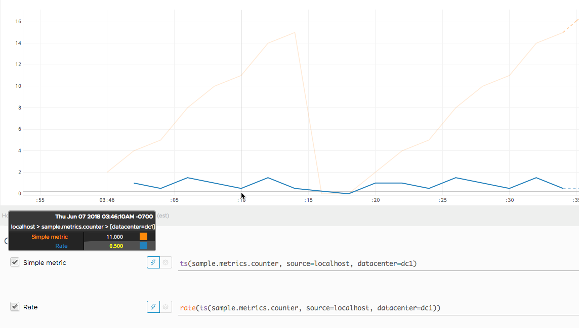
Figure 1. A Wavefront rendered graph of the random walk counter.

Representing a counter without rate normalization over some time window is rarely useful, as the representation is a function of both the rapidity with which the counter is incremented and the longevity of the service. It is generally most useful to rate-normalize these time series to reason about them.

Because Wavefront keeps track of cumulative counts across all time, it has the advantage of allowing for the selection of a particular time function at query time (for example, rate(ts(counter)) to compute the per-second rate of change).

3.2. Timers

The Wavefront Timer produces different time series depending on whether or not publishPercentileHistogram is enabled.

If publishPercentileHistogram is enabled, the Wavefront Timer produces histogram distributions that let you query for the latency at any percentile using hs() queries. For example, you can visualize latency at the 95th percentile (percentile(95, hs(timer.m))) or the 99.9th percentile (percentile(99.9, hs(timer.m))). For more information on histogram distributions, see Wavefront Histograms, later in this section.

If publishPercentileHistogram is disabled, the Wavefront Timer produces several time series:

${name}.avg: Mean latency across all calls.
${name}.count: Total number of all calls.
${name}.sum: Total time of all calls.
${name}.max: Max latency over the publishing interval.
${name}.percentiles: Micrometer-calculated percentiles for the publishing interval. These cannot be aggregated across dimensions.

You can use these time series to generate a quick view of latency in Wavefront:

Figure 2. Timer latency.

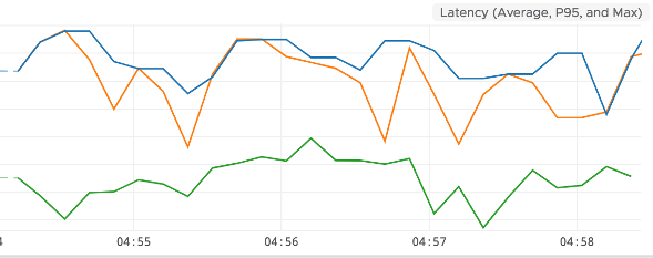
The preceding chart shows the average latency (rate(ts(timer.sum))/rate(ts(timer.count)) in green), 95th percentile (ts(timer.percentile, phi="0.95") in orange), and max (ts(timer.max) in blue).

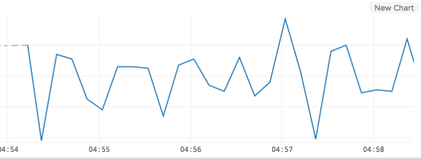
Additionally, rate(ts(timer.count)) represents a rate/second throughput of events being timed:

Figure 3. Timer throughput.

3.3. Wavefront Histograms

Wavefront’s histogram implementation stores an actual distribution of metrics, as opposed to single metrics. This lets you apply any percentile and aggregation function on the distribution at query time without having to specify specific percentiles and metrics to keep during metric collection.

Wavefront histogram distributions are collected and reported for any Timer or DistributionSummary that has publishPercentileHistogram enabled.

By default, distributions that are reported to Wavefront get aggregated by the minute, providing you with a histogram distribution for each minute. You also have the option of aggregating by hour or day. You can customize this with the following configuration options:

reportMinuteDistribution: Boolean specifying whether to aggregate by minute. Enabled by default. Metric name in Wavefront has .m suffix.
reportHourDistribution: Boolean specifying whether to aggregate by hour. Disabled by default. Metric name in Wavefront has .h suffix.
reportDayDistribution: Boolean specifying whether to aggregate by day. Disabled by default. Metric name in Wavefront has .d suffix.

If you are sending to a Wavefront proxy, by default, both metrics and histogram distributions are published to the same port: 2878 in the default proxy configuration. If your proxy is configured to listen for histogram distributions on a different port, you can specify the port to which to publish by using the distributionPort configuration option.

You can query histogram distributions in Wavefront by using hs() queries. For example, percentile(98, hs(${name}.m)) returns the 98th percentile for a particular histogram aggregated over each minute. Each histogram metric name has a suffix (.m, .h, or .d), depending on the histogram’s aggregation interval.

See the Wavefront Histograms documentation for more information.